Forecasting and Econometric Models
By Saul H. Hymans

An econometric model is one of the tools economists use to forecast future developments in the economy. In the simplest terms, econometricians measure past relationships among such variables as consumer spending, household income, tax rates, interest rates, employment, and the like, and then try to forecast how changes in some variables will affect the future course of others.
Before econometricians can make such calculations, they generally begin with an economic model, a theory of how different factors in the economy interact with one another. For instance, think of the economy as comprising households and business firms, as depicted in Figure 1. Households supply business firms with labor services (as tailors, accountants, engineers, etc.) and receive wages and salaries from the business firms in exchange for their labor. Using the labor services, businesses produce various outputs (clothing, cars, etc.) that are available for purchase. Households, using the earnings derived from their labor services, become the customers who purchase the output. The products the businesses produce wind up in the households, and the wage and salary payments return to the businesses in exchange for the products the households purchase.
This chain of events, as shown by the activities numbered 1–5 in Figure 1, is a description—or diagrammatic model—of the operation of a private-enterprise economy. It is obviously incomplete. There is no central bank supplying money, no banking system, and no government levying taxes, building roads, or providing education or national defense. But the essentials of the economy’s private sector—working, producing, and buying products and services—are represented in a useful way in Figure 1.

The diagrammatic model of Figure 1 has certain disadvantages when it comes to representing quantities such as the value of the wage and salary payments or the number of cars produced. To represent magnitudes more conveniently, economists employ a mathematical model, a set of equations that describe various relationships between variables. Consider household purchases of output, shown as activity 4 in Figure 1. If W is the value of the wages and salaries households earn, and C is household expenditures on clothing, then the equation C = .12W states that households spend 12 percent of their wages and salaries on clothing. An equation could also be constructed to represent household purchases of cars or any other goods and services. Indeed, each of the activities pictured in Figure 1 can be represented in the form of an equation. Doing so may take a blend of economic theory, basic economic facts about the particular economy, and mathematical sophistication; but once done, the result would be a mathematical or quantitative economic model, which is but one important step away from an econometric model.
In the equation for clothing purchases, C = .12W, “12 percent” was selected purely for illustrative purposes. But if the model is to say anything useful about today’s American economy, it must contain numbers (econometricians and others applying similar statistical methods refer to such numbers as “parameters”) that describe what actually goes on in the real world. For this purpose, we must turn to the relevant historical data to find out what percentage of household income Americans do, in fact, typically spend on clothing.
The column headed “Total” in Table 1 shows the percentage of (after-tax) income Americans spent on clothing (including shoes) for each of the years 1995–2002. One fact is immediately obvious: 12 percent was way off. If it had been left in the model, it would have led to a substantial overestimate of clothing purchases and would have been useless to understand or predict behavior in the American economy. Something closer to 4.21 percent, the average of the annual values in the “Total” column, would more accurately reflect total annual spending on clothing and shoes as a percentage of household income in the United States.
|
|
||
| % of Household Income | ||
| Year | Total | Total – 100 |
| 1995 | 4.5 | 2.6 |
| 1996 | 4.4 | 2.6 |
| 1997 | 4.3 | 2.6 |
| 1998 | 4.2 | 2.7 |
| 1999 | 4.3 | 2.8 |
| 2000 | 4.1 | 2.7 |
| 2001 | 4.0 | 2.6 |
| 2002 | 3.9 | 2.6 |
| Average | 4.21 | 2.65 |
|
|
||
A more careful look at the facts, however, reveals that 4.21 percent may not adequately represent the actual behavior. There has been substantial annual variation—from as much 4.5 percent to as little as 3.9 percent—in household income spent on clothing and shoes. What is more, there appears to be a downward trend, with the larger percentages coming in the mid-1990s and the smaller percentages coming more recently. The following simple statistical procedure takes care of these objections. Start with total annual spending on clothing and shoes, subtract $100 billion, and then calculate the balance—annual spending on clothing and shoes beyond the first $100 billion—as a percentage of household income. The column headed “Total − 100” in Table 1 shows the result—a very satisfactory result, with little annual variation around the average of 2.65 percent and no apparent trend over time.
You might well wonder what this subtraction of $100 billion represents. Here is a useful way to think about it. The U.S. population averaged 277.6 million persons during 1995–2002. Therefore, the value $100 billion represents, in round numbers, $360 per person ($100 billion divided by 277.6 million persons). The facts in Table 1 suggest that an expenditure on clothing and shoes averaging about $360 per person per year is a base, or minimally acceptable, amount in the United States these days. Once that minimum is accounted for, additional purchases of clothing and shoes will amount to 2.65 percent of household income.
In other words, Americans spend more on clothing and shoes the higher their household income, but they spend at least $100 billion per year. And the best forecast of the total that will be spent is: $100 billion plus an additional 2.65 percent of household income. In equation form, this is represented by C = 100 + .0265W, a far cry from the C = .12W we began with. The fact that the parameter values 100 and .0265 in the clothing equation were determined by using the relevant data is what gives us reason to believe that the equation says something meaningful about the economy. Using the data to determine or estimate all the parameter values in the model is the critical step that turns the mathematical economic model into an econometric model.
An econometric model is said to be complete if it contains just enough equations to predict values for all of the variables in the model. The equation C = 100 + .0265W, for example, predicts C if the value of W is known. Thus, there must be an equation somewhere in the model that determines W. If all such logical connections have been made, the model is complete and can, in principle, be used to forecast the economy or to test theories about its behavior.
Actually, no econometric model is ever truly complete. All models contain variables the model cannot predict because they are determined by forces “outside” the model. For example, a realistic model must include personal income taxes collected by the government because taxes are the wedge between the gross income earned by households and the net income (what economists call disposable income) available for households to spend. The taxes collected depend on the tax rates in the income tax laws. But the tax rates are determined by the government as a part of its fiscal policy and are not explained by the model. If the model is to be used to forecast economic activity several years into the future, the econometrician must include anticipated future tax rates in the model’s information base. That requires an assumption about whether the government will change future income tax rates and, if so, when and by how much. Similarly, the model requires an assumption about the monetary policy that the central bank (the Federal Reserve System in the United States) will pursue, as well as assumptions about a host of other such “outside of the model” (or exogenous) variables in order to forecast all the “inside of the model” (or endogenous) variables.
The need for the econometrician to use the best available economic judgment about “outside” factors is inherent in economic forecasting. An econometrically based economic forecast can thus be wrong for two reasons: (1) incorrect assumptions about the “outside” or exogenous variables, which are called input errors; or (2) econometric equations that are only approximations to the truth (note that clothing purchases beyond the minimum do not amount to exactly 2.65 percent of household income every year). Deviations from the predictions of these equations are called model errors.
Most econometric forecasters believe that economic judgment can and should be used not only to determine values for exogenous variables (an obvious requirement), but also to reduce the likely size of model error. Taken literally, the equation C = 100 + .0265W means that “any deviation of clothing purchases from 100 plus 2.65 percent of household income must be considered a random aberration from normal or expected behavior”—one of those inherently unpredictable vagaries of human behavior that continually trip up pollsters, economists, and others who attempt to forecast socioeconomic events.
The economic forecaster must be prepared to be wrong because of unpredictable model error. But is all model error really unpredictable? Suppose the forecaster reads reports that indicate unusually favorable consumer reaction to the latest styles in clothing. Suppose, on this basis, the forecaster believes that next year’s clothing purchases are likely to exceed the usual minimum by something closer to 3 percent than to the usual 2.65 percent of household income. Should the forecaster ignore this well-founded belief that clothing sales are about to “take off,” and thereby produce a forecast that is actually expected to be wrong?
The answer depends on the purpose of the forecast. If the purpose is the purely scientific one of determining how accurately a well-constructed model can forecast, the answer must be: Ignore the outside information and leave the model alone. If the purpose is the more pragmatic one of using the best available information to produce the most informative forecast, the answer must be: Incorporate the outside information into the model, even if that means effectively “erasing” the parameter value .0265 and replacing it with .0300 while generating next year’s forecast. Imposing such “constant adjustments” on forecasts was at one time disparaged as entirely unscientific. These days, many researchers regard such behavior as inevitable in the social science of economic forecasting and have begun to study how best—from a scientific perspective—to incorporate such outside information.
Much of the motivation behind trying to specify the most accurately descriptive economic model, trying to determine parameter values that most closely represent economic behavior, and combining these with the best available outside information arises from the desire to produce accurate forecasts. Unfortunately, an economic forecast’s accuracy is not easy to judge; there are simply too many dimensions of detail and interest. One user of the forecast may care mostly about the gross domestic product (GDP), another mostly about exports and imports, and another mostly about inflation and interest rates. Thus, the same forecast may provide very useful information to some users while being misleading to others.
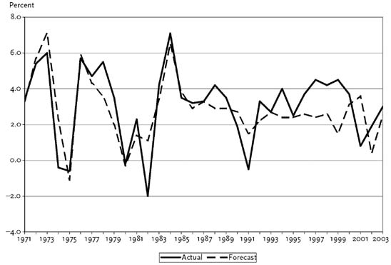
For want of anything obviously superior, the most common gauge of the quality of a macroeconomic forecast is how accurately it predicts real GDP growth. Real GDP is the most inclusive summary measure of all the finished goods and services being produced within the geographic boundaries of the nation. For many purposes, there is much value in knowing with some lead time whether to expect real GDP to be increasing at a rapid rate (a booming economy with a growth rate above 4 percent), to be slowing down or speeding up relative to recent behavior, or to be slumping (a weak economy with a growth rate below 1 percent or even a recessionary economy with a negative growth rate). The information contained in Figure 2 can be used to judge, in the summary fashion just indicated, the econometric forecasting accuracy achieved by the Research Seminar in Quantitative Economics (RSQE) of the University of Michigan over the past three-plus decades.
The RSQE forecasting project, dating back to the 1950s, is one of the oldest in the United States. Figure 2 compares, for each of the years 1971–2003, the actual percentage change in real GDP (the economy’s growth rate) with the RSQE forecast published in November of the preceding year. There are several ways to characterize the quality of the RSQE forecasting record. Although the forecasts missed the actual percentage change by an average of only 1.1 percentage points (measured by the average forecast error without regard to sign), the forecast error was as small as 0.5 percentage point or less in thirteen of the thirty-three years shown. On the other hand, six years had forecast errors of 2 percentage points or more, and for 1982 and 1999, the forecast errors were 3.1 and 3.0 percentage points, respectively. But, despite some relatively large errors, there was never a boom year that RSQE forecast to be a weak year; never a weak year that RSQE forecast to be a boom year; and just a few instances—most recently, 1999 and 2001—in which the forecast really went “the wrong way” in the sense of missing badly on whether the economy’s growth rate was about to increase or decrease relative to the preceding year’s growth rate.
The discussion, so far, has focused on what is referred to as a structural econometric model. That is, the econometrician uses a blend of economic theory, mathematics, and information about the structure of the economy to construct a quantitative economic model. The econometrician then turns to the observed data—the facts—to estimate the unknown parameter values and turn the economic model into a structural econometric model. The term “structural” refers to the fact that the model gets its structure, or specification, from the economic theory that the econometrician starts with. The idea, for example, that spending on clothing and shoes is determined by household income comes from the core of economic theory.
Economic theories are both complex and incomplete. To illustrate:
•
Does this year’s spending on clothing depend only on this year’s income or also on the pattern of income in recent years?
•
How many years is “recent”?
•
Don’t other variables, such as the price of clothing relative to other consumer goods, matter as well?
This situation makes it far more difficult than implied to this point to specify the economic model one must begin with to wind up with a structural econometric model for use in forecasting. In recent years, econometricians have found that it is possible to do economic forecasting using a simpler, nonstructural, procedure without losing much forecast accuracy. Although the simpler procedure has significant costs, these costs do not show up in the normal course of forecasting. This will be explained after a quick introduction to the alternative procedure known as “time-series forecasting.”
The idea of time-series forecasting is easily explained with the aid of Figure 3, which shows year-by-year changes in spending on clothing and shoes starting in 1981 and

going through 2002. The horizontal line marks the average annual change of $8.8 billion.
Most of the year-to-year changes are in the range of $4.4–$13.2 billion, and only one change, that of 2001, is well outside that range. The year-to-year changes, in other words, appear to be stable. Some are above $8.8 billion and some are below; 1983–1988 exhibited a string of changes that were all close to $11 billion, but that was unusual. More often, one year’s change is little guide to the next year’s change, as the changes jump around too much. So, a forecasting rule that says next year’s spending on clothing and shoes will be $8.8 billion more than this year’s spending makes good sense. And that, for this simple case, is the essence of time-series forecasting. Look carefully at the historical behavior of the variable of interest, and if that behavior is characterized by some kind of stability, come up with a quantitative description of that stability and use it to construct the forecast.
It is not always easy to “see” the stability that can be counted on to provide a reliable forecast, and econometricians have developed sophisticated procedures to tease out the stability and measure it. In general, the time-series procedure and the structural model procedure seem to produce comparably good, or bad, forecasts for a year or two into the future. But the time-series procedure has the distinct advantage of being far simpler. We can forecast spending on clothing and shoes without having to worry about the theoretical relationship between spending and household income. It need not be specified and its parameters need not be estimated; just focus on the clothing variable itself.
So, where are the significant costs in using the time-series forecasting procedure? They come from the fact that the procedure gives a numerical answer and nothing else. If the user of the forecast—for example, a clothing manufacturer—asks why the forecast says what it does, the time-series econometrician can answer only, “Because that’s the way spending on clothing has behaved in the past,” not, “Because household income is going to rise sharply in response to an expansionary monetary policy which is being conducted in order to . . .” In short, there is no economics in the analysis in the first place. If there were, the user would be able to respond, “That makes sense; I’ll plan on the basis of the forecast”; or, alternatively, “I think that forecast is too good to be true because I’m convinced that expansionary monetary policy is about to be reversed, and so I’m shaving the forecast in my planning.” Time-series forecasting leaves the user “hanging”: just take it or leave it.
Because many forecasters work with structural models, users can acquire not only the various numerical forecasts, but also the economic analysis that accompanies and justifies, or explains, each forecast. A user who has to act on the basis of a forecast and can choose among the alternative forecasts available is surely getting much more information when those forecasts have a structural economic basis.
Finally, and related to the preceding discussion, structural models are the “only game in town” when it comes to the important area of econometric policy analysis or other “what if” calculations. Thus, a baseline forecast may be calculated using a structural econometric model and the best information available to the forecaster. And then someone asks, “What if Congress raises the income tax rate by five percentage points?” This single perturbation is then imposed on the original calculation, and the forecast is recalculated to show the model’s evaluation of the effect on the economy of the posited change in government fiscal policy.
Economists commonly employ such calculations in the process of providing advice to businesses and units of government. The practical validity of such applications depends on how well the model’s structure represents the economic behavior that is central to the “what if” question being asked. All models are merely approximations to reality; the issue is whether a given model’s approximation is good enough for the question at hand. Thus, making structural models more accurate is a task of major importance. As long as model users ask “what if,” structural econometric models will continue to be used and useful.
Further Reading