The Quantity Theory of Money in the Weimar Hyperinflation

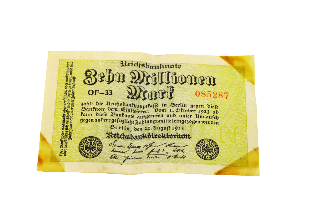
In my two previous posts (here and here) I described how hyperinflation hit the Weimar Republic after the end of World War 1. On November 15, 1923, the German Papiermark hit an exchange rate of 2.5 trillion to $1. Two weeks earlier, $1 had bought 133 billion marks; at the start of the year 17,972 marks; on the currency’s introduction in 1914, 4.19. Germany’s currency died. What killed it?  

We can begin to answer that question with the equation of exchange, only of the few genuinely useful equations in economics:

MV=Py

This says that the money supply in an economy (M) multiplied by the number of times it is spent in a given period (velocity of circulation, V) equals the price level (P) multiplied by output (y); nominal spending (MV) equals nominal income (Py).  

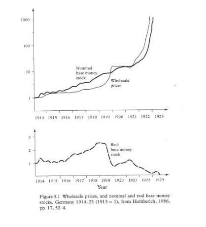
Assuming that V and y are fixed, it follows that any increase in M must lead to an increase in P: inflation. But in Germany in 1921-1923, Theo Balderston writes, “prices did not rise in step with the money supply as the quantity theory implies.” Instead, he notes that:

The quantity theory of money – as restated by Milton Friedman – can account for this, however. It incorporates the ‘demand for money,’ or the demand to hold cash balances. Balderston explains that holding money balances:

When those opportunity costs change, so does the demand for money. Besides the “‘opportunity cost’ of holding wealth as money balances in terms of the interest income foregone,” Balderston notes that:

They ‘economise’ by spending their balances: in other words, when the opportunity cost of holding money balances is perceived to rise, the demand for money falls, V increases, and p rises, even if M is kept constant. And, in reverse, when the opportunity cost of holding money balances is perceived to fall, the demand for money rises, V decreases, and p falls, even if M is kept constant. 

Data on the forward exchange rate of the mark from 1921 do show a stable, negative relationship between expected inflation and the real demand for money. What drove expectations? Carl-Ludwig Holtfrerich, Balderston notes, “connected expectational changes to reparations crises.” Germany was wrangling with the Allies over the terms of the Versailles Treaty which had concluded World War One. In April 1921, the Allies presented their bill. Seen as unpayable by most Germans, they believed the government would resort to printing money to meet its liabilities. The opportunity cost of holdings marks was perceived to rise and Germans sought to ‘economize’ on their mark holdings by spending them. Further fiscal pressures arising from the Franco-Belgian occupation of the Rhur in January 1923 exacerbated this.    

But there is a limit to this. The demand for real money balances cannot fall below a certain level because the time between acquiring money and spending it cannot be compressed to zero. By late 1922, Frank D. Graham argued, marks were being spent as fast as possible. This was the period of people running to the shops as soon as they received their wages. 

Thus, Balderston argues, “in the long run, inflation cannot persist if the money supply does not expand.” “In this final period,” he writes, “inflation was probably driven by the money-supply process” outlined by Steven B. Webb, who argued that inflation expectations prompted people to dump government debt which the central bank bought with newly printed money to keep government borrowing costs down.  

Milton Friedman famously argued that:

That description fits the Weimar hyperinflation, even if the story is a little more nuanced than that famous formulation suggests.