The Power to Tax: Analytical Foundations of a Fiscal Constitution

It will be useful to begin our discussion of commodity taxation with a brief review of the central elements of orthodox doctrine. This procedure will allow us to point up the contrasts between the standard normative results and those which emerge under the alternative constitutional perspective on taxation applied within a Leviathan or Leviathan-like model of political process. In commodity-tax analysis, as elsewhere in orthodox tax literature, the point of departure is some presumed requirement that government raise a fixed and exogenously determined amount of revenue. Given this fixed-revenue requirement, the question is: How should taxes be levied so as to minimize welfare loss? As noted earlier, the orthodox procedure is to attempt to answer this question independent of any consideration concerning the uses to which tax revenues may be put. This analytical weakness aside, the traditional argument has concentrated on the efficiency aspects of differing commodity-tax arrangements. Equity and/or distributional implications have been less emphasized in commodity-tax analysis than in income-tax analysis. The issue of the normatively desired form of commodity taxation has been treated largely as a problem of minimizing excess burden, with some consideration of horizontal equity (i.e., of avoiding discrimination among individuals on the basis of tastes or other “irrelevancies”). Vertical equity issues have tended to be effectively ignored. The literature has noted the equivalence between a uniform tax on all commodities and a personal tax on consumption expenditure with a proportional rate structure;
*46 nonetheless, within the indirect tax analysis, as such, the concentration has remained on the efficiency properties of alternative tax arrangements.

Basically, the application of the same normative framework to both commodity and income taxes tends to generate policy recommendations of the same type and direction. Personal taxes should allegedly be broadly based so that there is no (or minimal) discrimination among individuals on the basis of how income is earned; similarly, commodity taxes should allegedly also be broadly based—and ideally should tax all “goods,” including leisure, equally—so as to minimize discrimination among individuals on the basis of how income is spent. Likewise, just as failure to tax all income sources equally under direct taxation is adjudged to lead to efficiency losses as individuals attempt to substitute less productive but relatively lightly taxed activities for those more highly taxed, so failure to tax all
goods equally under commodity taxation is taken to lead to efficiency losses on the consumption side.

In both cases, or so says the prevailing tax-analysis orthodoxy, lump-sum taxation represents the idealized benchmark. Given the infeasibility or even the impossibility of lump-sum taxation, the practical question necessarily becomes one of selection among second-best options. Whereas with personal taxes the “second-best” arrangement is normally assumed to be the broadest-based income tax (or consumption-expenditure tax) that is feasible, with indirect taxes the possibility of using differential rates on goods according to their degree of complementarity with leisure (relatively high rates on leisure complements, and lower rates on goods relatively highly substitutable with leisure) naturally presents itself. As emphasized by Corlett and Hague, Harberger, Lerner, Baumol, and Bradford and in much of the “optimal-taxation” literature in general,
*47 a set of differential excises can be devised that involves a smaller welfare loss or “excess burden” than does an equi-revenue tax falling equally on all the directly taxable commodities (i.e., excluding leisure).
*48 It is always more efficient to raise a given amount of revenue by means of a set of taxes in which the tax rate applied to each good is appropriately related to the degree of substitutability between that good and the untaxed good, leisure, than by an equal rate on all taxed goods.
*49

4.2. Constitutional Tax Choice

As in our discussion of income taxation, our quarrel is not with the
logic of the orthodox conclusions. It is, instead, with the
setting within which the questions are posed. Once the implicit “benevolent dictator” conception of political process is rejected, the appropriate role for normative tax analysis becomes that of offering assistance to the individual, the potential taxpayer, who, at a constitutional level of deliberation, is presumed able to select among the alternative fiscal powers and instruments to be made available to government. Such assistance is not, however, in the form of ethical-moral principles telling the individual how he “should” behave in a constitutional choice situation. For the most part, constitutional tax analysis becomes technical and is designed to provide a basis for an understanding of how alternative fiscal arrangements may be predicted to operate, a basis from which some choice must ultimately be made.

Given a model of revenue-maximizing government, the implied normative conclusions about commodity taxation follow the spirit of those outlined in Chapter 3. And they are diametrically opposed to those that emerge from the standard treatment. For example, the lump-sum tax does not constitute the “efficiency” ideal. Under lump-sum taxation, the individual can expect only maximum exploitation by the fisc. Under almost any projection of demands, revenue collections would be predicted to be grossly in excess of those that might be required to finance expenditures on public goods and services. In much the same sense, the minimally distorting set of excises (i.e., with rates related inversely to the degree of substitutability with leisure) serves to raise maximum revenue limits above those implied by a uniform commodity tax and almost certainly to increase total revenue beyond desired levels. Indeed, a restriction that all rates on taxable commodities be identical might well be instituted precisely as a means of restricting Leviathan’s fiscal appetites.

In the more formal analysis that follows, we offer analytic support for these conclusions. More specifically, we deal with two sorts of questions. First, what are the effects on maximum revenue yield of alternative forms of restriction on commodity-tax institutions? Second, given a choice among various forms of commodity tax all of which yield the same maximum revenue, which, if any, is to be preferred?

4.3. Alternative Forms of Commodity Tax: The Choice of Base

We classify the alternative forms of commodity taxation to be examined in terms of the restrictions on allowable arrangements—whether base restrictions, restrictions on rate structure, requirements for uniformity across commodities, or requirements for uniformity across individuals and over units.

Figure 4.1

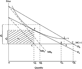
The discussion can be conducted conveniently in terms of the diagrammatics of Figure 4.1. In this diagram,
D
_a and
D
_b represent the aggregate (market) demand curves for two private, partitionable goods,
A and
B. These demand curves are assumed to be linear for expositional convenience, and cost curves are horizontal to reflect constant average (and hence marginal) costs. Quantity units are defined so that the initial marginal cost (assumed equal to price) is unity.

Let us suppose that
A and
B represent the only potential tax bases that might be assigned to government. The individual’s constitutional choice between them depends directly on the estimated needs for financing the quantity of public goods and services that he expects to desire over the sequence of budgetary periods during which the selected tax rule is to remain in force. If government is assigned the authority to tax
A, it will, under Leviathan assumptions, maximize the revenue it can obtain from taxes on this base. The power to tax commodity or good
A is identical analytically to the assignment of a monopoly franchise for the sale of commodity
A. As depicted in Figure 4.1, the revenue maximum occurs at
Q_a*, the quantity defined by the intersection between the marginal revenue curve,
MR
_a, and the marginal cost curve,
MC. The revenue-maximizing tax rate is
t_a*; revenue collected is
t_a*
Q_a*, shown by the shaded area.

It is clear from the construction in Figure 4.1 that if the tax on commodity
A is replaced by a tax on commodity
B, the same amount of revenue could be obtained at a lower tax rate and a smaller excess burden. Let
r be a rectangular hyperbola with the ordinate and the horizontal
MC line as its axes, and let
r pass through
F. Every price-quantity combination along
r, by construction, yields the same tax revenue (“monopoly profit”) as at
F. Since
F is the point at which maximum tax revenue is obtainable from
A, r must be tangent to
D
_a at
F. Now, consider point
L, at which
r intersects with
D
_b (to the right of
F).
*50 At
L, the same revenue that is obtained by the maximum revenue tax on
A could be obtained by a tax of rate
LS imposed on
B. The welfare loss imposed by such a tax on
B is
LST, which is much smaller than the welfare loss
FCE imposed by the tax on
A. Hence, the traditional efficiency or welfare argument for the broader-based tax seems to emerge.

Under the assumptions about the behavior of government that we have made, however, it is clear that a tax rate of
LS will not be imposed on commodity
B. If government is granted access to base
B, with no accompanying restriction on rates, this change will ensure that there will be an increase in the revenue that government will appropriate. Government will secure the maximum revenue obtainable from the tax on
B. This revenue is
t_b*
Q_b* in Figure 4.1, where
Q_b* is determined by the intersection of
MR
_b and
MC, and
t_b* is the excess of demand price over
MC at that quantity. It is clear that, under these conditions, the excess burden will be larger under the tax on
B than the tax on
A. Under the assumptions of proportional rate structure and linear demand curves,
*51 the excess burden induced by a tax exploited to its maximum revenue potential is exactly one-half the maximum revenue raised. A simple geometric proof of this proposition suffices at this point in the argument. All we need to note is that in the linear case, the marginal revenue curve lies exactly halfway between the demand curve and the vertical axis. In Figure 4.1,
Q_a* is exactly one-half
Q
_a. The area of the triangle
CEF in Figure 4.1 is given by ½ (
t_a* ·
CE); and since
CE equals
Q_a*, the welfare-loss triangle
CEF is ½ (
t_b*
Q_a*), or one-half of maximum revenue. Analogously, since
Q_b* is exactly one-half of
Q
_b, the welfare loss attributable to the maximum revenue tax on
B is ½
t_b* · (
Q
_b –
Q_b*) or ½ (
t_b*
Q_b*). We can conclude therefore that the ratio of excess burdens induced by alternative taxes will be the same as the ratio of their maximum revenue yields: if tax
B generates larger maximum revenue than tax
A, then it will generate a concomitantly larger excess burden when maximum revenue yields are obtained.

Figure 4.2

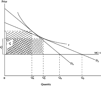
An immediate corollary of this result is that if we compare two taxes with identical maximum revenue yields under a proportional rate structure, they will generate identical excess burdens (given the appropriate linearity assumptions). Consider, for example, a commodity-tax base,
X, which, when used to generate maximum revenue, yields the same maximum revenue as does tax base
Y. Any number of such tax bases may exist, but a simple direct comparison of any two of them will suffice to make the point. As before, let
D
_x and
D
_y depict the aggregate demand curves for these alternative tax-base commodities in Figure 4.2. The maximum revenue rates produce identical revenues. The solutions represent differing points along the rectangular hyperbola,
r. Is either one of these taxes to be preferred on the grounds that it generates a lower excess burden? Since both generate the same maximum revenue, and since the welfare loss at maximum revenue rates is one-half of maximum revenue in both cases,
the excess burdens as well as the maximum revenues are identical. In other words, in this construction if we compare proportional taxes that raise the same maximum revenue, there can be no preference between them on excess burden grounds. Maximum revenue itself becomes a sufficient indicator of excess burden, as conventionally measured.
*52

A further corollary of this result is that if we compare two tax bases which are of identical magnitude pretax but for which elasticities of demand differ, the one with the lower elasticity of demand will give rise to the
larger excess burden, because it gives rise to a larger maximum revenue. (Geometrically, this comparison could be depicted in a diagram similar in construction to
Figure 3.3, with the demand curves of persons replaced by those for commodities.) This result is diametrically opposed to that which emerges from the conventional equi-revenue approach, which relates excess burden directly with elasticity.

If there can be no preference for broad-based taxes derived from excess burden comparisons (rather the contrary) within our Leviathan setting, the choice between broad- and narrow-based taxes—say, between a tax on
A and a tax on
B, as depicted in Figure 4.1—depends solely on the level of public-goods supply which the citizen expects to want. This anticipated desired level of public-goods supply depends in turn on both the predicted demand for public goods and on the total cost of providing them.

Figure 4.3

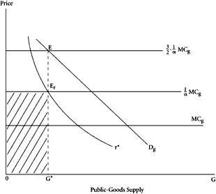
Consider total cost first. These costs are composed of three elements, as illustrated geometrically in Figure 4.3. First, there is the physical cost of production of
G, depicted in marginal terms by
MC
_g (which again for convenience we assume to be constant). Second, there is the additional cost imposed by the Leviathan government’s appropriation of some proportion, 1 –
a, of tax revenue as pure surplus. If, out of each dollar of revenue, only 100
a cents are expended on public goods, then the total revenue cost of $1’s worth of
G is 1/
a dollars. If government, for example, spends only one-half of each revenue dollar on providing
G, then each dollar’s worth of
G will cost taxpayers $2 in tax revenue. This ”
a effect” raises the per unit cost of
G to 1/
aMC
_g, as indicated in Figure 4.3. Third, there is the excess burden generated by the tax itself, which is also a genuine cost. As indicated above, given linear demand schedules and constant costs, and with proportional rates imposed at maximum revenue levels, this excess burden will be exactly one-half of (maximum) revenue. The aggregate cost per dollar’s worth of
G will then be 3/2 1/
aMC
_g, depicted in Figure 4.3.

The desired level of
G, given this aggregate cost, can now be determined by appeal to the typical citizen’s constitutional predictions as to his demand for public goods. We should emphasize at this point that there is no necessary requirement here that all citizens have identical predicted demands for public goods (although in a strict veil-of-ignorance setting such an assumption would not be particularly implausible: to the extent that each individual is totally uncertain as to his future tastes and income level, we might expect that predicted demands for public expenditures on
G would be roughly identical across individuals). It is sufficient here, however, to focus on the calculus of a single typical citizen. To consider the additional problems involved in deriving some constitutional agreement among citizens on the issue of appropriate tax allocations to Leviathan in the case where those citizens have differing predicted demands for
G would complicate the discussion and divert us from our main purpose.

Let us depict the typical citizen’s predicted demand for
G by
D
_g in Figure 4.3. Where this demand curve cuts the aggregate marginal cost line, 3/2 1/
aMC
_g, will determine the desired level of
G, depicted by
G*. The level of
revenue required to generate this output level,
G*, is 1/
aMC ·
G*, because
MC ·
G* is the physical cost of producing
G* and
a is the proportion of revenue that Leviathan spends on
G. This revenue level is depicted by the shaded rectangle in Figure 4.3. We can now, finally, construct a rectangular hyperbola through
E
_r, depicted by
r*, which depicts the desired level of (maximum) revenue.

The virtue of this diagrammatic treatment is that it permits us to show on a single diagram and in a neat and simple way the interrelationships among the citizen’s demand for public goods; the cost of physically producing those public goods; the “exploitative” dimensions of Leviathan’s surplus generation, as captured by the parameter,
a; the excess burden generated by the tax system;
*53 and the desired level of (maximum) revenue potential to which the constitution will permit Leviathan access.

Since our main interest here is with the constitutional selection of tax instruments, we focus directly on that issue. What we seek in the selection of the appropriate commodity-tax base is a base that will, when exploited to its maximum revenue potential, yield exactly that revenue which is required to generate
G* (i.e., a revenue level subtended by any rectangle under
r*). Suppose, for the purposes of argument, that the tax base
A does this. In other words, suppose that the level of tax revenue indicated by
r* in Figure 4.3 is exactly the same as that indicated by
r in Figure 4.1. (Geometrically, this requires that if Figure 4.3 were superimposed on Figure 4.1 so that the abscissa in Figure 4.3 lay along the
MC line in Figure 4.1 and so that the vertical axes were collinear, then
r and
r* would be coincident.) Then, if tax base
A is in use, it follows that any broadening of the tax base would be undesirable. Such a broadening would lead to a higher level of tax revenues and of public-goods supply than the citizen-taxpayer desires, given the particular values of
a and
MC
_g as shown in Figure 4.3. To select, for example, the tax base
B would generate a maximum revenue level above that depicted by
r*, a corresponding level of
G above
G*, and leave the citizen predicting excessive exploitation by government in postconstitutional periods, along with unnecessarily high welfare losses in the tax system. At the same time, any tax base that generates the same maximum revenue as can be derived from a tax on
A is equally acceptable with
A. Within that set of tax options which yield identical maximum revenue, the citizen-taxpayer is genuinely indifferent.

What this discussion shows can be encapsulated in two statements: first, greater broadness of coverage under commodity taxation is not unambiguously desirable and it is positively undesirable beyond some point; and second, excess burden varies directly and linearly with maximum revenue, so that taxes which have identical maximum revenue have identical excess burdens when maximum revenue rates are applied, and taxes with larger maximum revenue yield a larger excess burden when maximum revenue rates are used (and vice versa). Base limitation therefore emerges as a legitimate instrument in the design of tax constitution for a Leviathan government. The general thrust toward broader-based tax institutions, characteristic of the orthodox analysis, cannot be sustained within the alternative perspective on tax institutions that we postulate in this book.

4.4. Uniformity of Rates over Commodities

Let us now suppose that, maintaining the basic assumptions of the previous section, the maximum revenue realized from taxation of
A or
B is insufficient to provide the level of public-goods supply anticipated to be desired during the postconstitutional sequence. The question then arises as to how government might be granted authority to tax
both A and
B, in order to secure the required revenue. If we assume that specific rates for each commodity cannot be set in advance, essentially two tax-structure possibilities present themselves. Government may be constrained to set the
same rate on both
A and
B, or it may be allowed to set the rates on commodity
A and commodity
B independently and separately. In other words, Leviathan may be allowed access to a “uniform” sales tax which includes
A and
B in the base; or it may be permitted to apply a set of discriminatory excises, with rates of its own choosing.

Figure 4.4

In the latter case, if we assume that
A and
B are two of a large number of commodities and neither complements or substitutes one for another, a change in the price of
A does not directly affect the price of
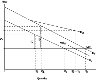
B, and vice versa. In this setting, it is clear that a revenue-maximizing Leviathan will set the tax rate on
A at
t_a*, as depicted in Figure 4.4, and the tax rate on
B at
t_b*.

If, by comparison, government is constrained to set a uniform rate for both commodities, it is necessary to aggregate the demand curves in order to depict its revenue-maximizing solution. Our construction in which quantity units for the two goods are normalized in the dollar’s worth dimension facilitates the aggregating of heterogeneous commodities. We can, quite simply, add the demand curves for the two commodities horizontally, to get the curve
D
_ab, as shown in Figure 4.4. Given the rate-uniformity constraint, government will set the tax rate so as to generate the quantity determined by the intersection between the marginal revenue curve relevant to the aggregated demand curve and the marginal cost curve. This solution is depicted in Figure 4.4 at quantity ½(
Q
_b +
Q
_a), with tax rate
t* imposed uniformly on each of the two commodities. Given the assumptions of linear demand and constant marginal cost curves, total quantity, over the two goods, remains constant as between rate uniformity and rate differentiation. This constancy result emerges from the simple geometrical configuration. Since
Q_a* (the quantity of
A under discriminatory rates) is ½
Q
_a, and
Q_b* (the quantity of
B under discriminatory rates) is ½
Q
_b, the aggregate quantity under the discriminatory solution is ½ (
Q
_a +
Q
_b). But this quantity is identical to that which emerges in the nondiscriminatory solution. However, given that
t_b* >
t_a*, the quantity of
B will be lower in the discriminatory solution than in the uniform-rate solution; conversely, the quantity of
A will be higher in the discriminatory solution than in the uniform-rate solution. The revenue-maximizing uniform rate of tax,
t*, will lie between the two separate revenue-maximizing rates,
t_a* and
t_b*, in the discriminatory solution.

The maximum revenue yield to government is higher in the discriminatory than in the uniform-rate situation as long as the elasticities of demand for the two commodities differ and as long as positive revenues are obtained from both commodities in the uniform-rate solution. Under such conditions, by our earlier analysis, it follows that excess burden is also lower under the uniform-rate requirement than in the situation where differential revenue-maximizing rates may be set. These results are, of course, familiar and become obvious once one accepts the analogy between the granting of the power to tax a commodity and the granting of a monopoly franchise. The requirement for uniform rates of tax for separate commodities is precisely analogous to the prevention of discrimination in monopoly price over separate segments of a market.
*54

The connection between these aspects of our analysis and the optimal-tax literature here is interesting. Reinterpreted within the setting of our model, what the so-called “optimal-taxation” literature provides is a specific set of instructions to government as to how it might exploit its power to tax in the most effective way. The analysis provides precisely that tax-price rule which would lead a monopolist to discriminate perfectly between markets.
*55 In this context, the optimal-tax rules are
precisely the maximum revenue-maximum profit rules. The analogy is evident here, but it has not, to our knowledge, been specifically noted.

The diagrammatic analysis we have employed is, to be sure, strictly partial—no allowance is made for the interaction between the demand for
A and the price of
B, and vice versa. It could therefore be claimed that it hardly bears on the optimal-tax literature, which typically adopts a general equilibrium framework. But the foregoing discussion can easily be extended to a general equilibrium setting; such an extension is provided in the appendix to this chapter.

We have, in this section, referred to differing rates of tax on differing commodities as “discrimination,” partially to emphasize the analogy with discriminatory monopoly. This construction is made more tenable by our normalization of quantity units for separate commodities in the “dollar’s worth” dimension. Nonetheless, we should acknowledge that economists conventionally do not apply the term “discrimination” with reference to relative tax treatment of observably different commodity bases. The language of this section can be modified to conform with conventional usage by referring only to uniform and nonuniform rates of tax.

There is an additional argument that may be adduced in support of conventional language here, an argument that has some relevance for the analysis of the following sections. As we know from orthodox price theory, a private monopoly firm may find it difficult to differentiate among customers or over units because of resale-retrading prospects. However, a monopoly firm that markets two separate and unrelated commodities would face little difficulty in setting different prices, even if quantity units are normalized in dollar-cost terms. In considering the differential rates of tax among commodities that governments may levy, we are analyzing a situation analogous to the monopoly firm in the second of these situations. By contrast, when we come to examine the prospects of tax-rate differentiation among persons or over units of goods, we look directly at the analogues to various forms of discriminatory monopoly.

4.5. Uniformity of Rates over Individuals

It would in principle be possible for optimal-tax recommendations to extend to the discriminatory treatment of different individuals. The simple partial equilibrium diagrammatics in Figure 4.4 are applicable,
*56 as was indeed indicated by our usage of essentially the same construction in Chapter 3 in Figure 3.3. By reinterpreting
D
_a and
D
_b in Figure 4.4 as the demand curves of two individuals for some taxable commodity
X, and
D
_ab as the aggregate demand over the “market” comprised of these two persons, we can derive the following results:

1. Consistent with the optimal-tax approach, any given level of revenue,
R, could be obtained with a smaller welfare loss by the appropriately discriminatory pattern of taxes—a relatively higher rate of tax on individual
B than on
A.

2. Equally and for precisely the same reasons, the maximum revenue potential increases when this pattern of discrimination is used.

3. If the maximum revenue potential is fully exploited, the welfare loss is concomitantly higher when discrimination among individuals is allowed.

As in the income-tax setting, therefore, the restriction that there be no discrimination among individuals on the basis of different tastes—one aspect of traditional horizontal equity norms—can be understood and justified in this setting as one limit on the revenue capabilities of Leviathan government.

We suggested that such possibilities for discrimination in rates among separate taxpayers exist “in principle” and that, if exploited, such discrimination would produce the comparative results indicated. The analysis requires the qualification noted at this point, however, because of the difficulty that even a monolithic and monopolistic Leviathan might confront in bridging the gap between “principle” and “practice.” In this particular respect, the analysis applied to income taxation (Chapter 3) becomes significantly different from that applied to commodity taxation (Chapter 4). Individuals must earn income on their own; they cannot readily work out arrangements by which other persons earn income on their behalf. By contrast, individuals need not purchase commodities directly. They can consume commodities purchased for them by others. And any differentiation among persons in rates of commodity tax (and hence in purchase price) sets up strong incentives for such indirect “purchases” to be made. For ordinary commodities, especially those that are not consumed on the instant of purchase, differential tax rates among different persons may prove impossible to implement. In practice, the effective rate of commodity tax would tend to be the lowest rate imposed on any person in the community, with this person becoming the direct purchaser for everyone. Imposition of a tax on final consumption rather than purchase of commodities might allow for rate differentiation, but monitoring costs would likely become prohibitive, even for the monopoly government. In a sense, therefore, the analysis of rate differentiation here among persons is more of an intellectual exercise than a treatment of a relevant prospect. The exercise itself, however, has the advantage of extending the direct analogy between monopoly government and the monopoly firm in traditional price theory. The institutional barriers to effective discrimination are equivalent in the two cases.

4.6. Discrimination by Means of the Rate Structure

We may extend this analogy between the taxing power and the monopoly franchise even further. If the ability to tax
X is identical with the power to sell
X at monopoly prices, it is clear that the best of all possible situations for Leviathan would be a situation in which tax rates might be set to mirror the price structure of the perfectly discriminating monopolist. In both cases, the idealized objective is to appropriate the full consumer surplus of each and every consumer. For purposes of analysis, let us ignore the practical difficulties noted above and examine two questions:

1. In our model of constitutional choice, what are the implications of perfect discrimination both among individuals and over units of the taxed commodities within the purchase opportunities of a given individual?

2. What if discrimination
over units is permitted but discrimination among individuals is not?

Figure 4.5

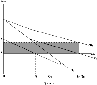
The “perfectly discriminatory” tax system.  We consider initially a simple two-person community, in which government has power to tax some good,
X, which we assume, as before, is produced under constant costs. The marginal evaluations of the two individuals for
X are depicted in Figure 4.5 by
D_I and
D_II.
*57 Under perfectly discriminatory taxes, each individual will face a different and regressive rate structure that traces out his or her marginal evaluation curve. The purchase-offer schedule will be designed to leave each individual with just enough consumer surplus to induce purchases up to the point where marginal evaluation equals marginal price, which will be set equal to marginal cost. For example, the tax-rate structure for I will begin with a rate marginally below
AK for the first unit of
X, and the rate will fall linearly with increases in
X consumption by I until the rate is zero at
Q_I. Similarly, for II the tax-rate structure will begin with a rate marginally below
AJ for the first unit of
X that II buys, and the rate will decline linearly to zero at
Q_II. Total revenue is given by the area under the aggregate demand curve for
X, the shaded area determined from the aggregate “average-revenue” schedule depicted as
AR
_x in Figure 4.5. This revenue is obtained without the imposition of any
excess burden.
*58

Figure 4.6

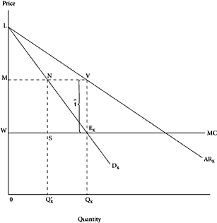
This relationship between rate discrimination and excess burden has implications that are worth exploring, even given the idealized confines of the model. To do so, we can ask the following question: If, under a uniform proportional tax on
X, the level of revenue is precisely that desired, could we be certain that allowing discrimination by means of the rate structure would be undesirable? For any other form of discrimination so far considered, the answer would be an unambiguous affirmative: discrimination would increase maximum revenue, increase excess burden, and push the level of public expenditure beyond the desired level. In this case, where the discrimination involves differentiation in rates over separate quantities of commodities purchased, however, the conclusion is not definitive. The move from the uniform proportional rate to the perfectly discriminatory set of regressive rates would, in the linear case, exactly double the revenue collected from each individual and hence the total revenue derived. It would, however, increase the costs endured by each citizen-taxpayer by only one-third (again assuming a linear demand curve for the taxed commodity). These propositions can be demonstrated by appeal to Figure 4.6. In the uniform nondiscriminatory tax case, the revenue derived from
X is the area
MNSW, representing
·
Q_x‘. Under this tax regime, the individual enjoys the net consumer surplus depicted by triangle
LMN. Consider the move to the discriminatory tax regime: the total revenue is here the full area of triangle
LWE
_x because all consumer surplus is appropriated by government in tax. Now, triangles
LMN and
NSE
_x are congruent, because
MN is equal to
WS, which is in turn equal to
SE
_x (i.e.,
Q_x‘ is exactly half of
Q
_x), and
MN and
SE
_x are parallel. Further, we know that
NSE
_x is exactly one-half the area of
MNSW. Hence,
LWE
_x has twice the area of
MNSW: revenue is twice as large in the perfectly discriminatory regime. And
LMN has an area equal to one-third of
MNE
_xW. We can therefore conclude that, in the move from uniform to perfectly discriminatory taxation, total revenue (and the level of public-goods supply) doubles, while aggregate costs rise by one-third. There has clearly been a reduction in the per unit cost to the citizen of public-goods supply. We know that

(1)

where
G is the level of public-goods supply,
R is the level of revenue derived by government, and the subscripts
d and
p refer to the perfectly discriminating and uniform outcomes, respectively. Further,

(2)

where
C is total cost to the citizen and equals the sum of excess burden and revenue.

Thus, the average cost, that is, the cost per unit of public good, which in this simple model is equal to marginal cost, varies in the two cases as follows:

(3)

Perfect discrimination reduces the
per unit cost of public-goods supply by one-third.

Figure 4.7

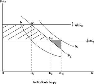
In short, perfect discrimination both increases the level of public-goods supply
and reduces the per unit cost of public-goods supply. In order to determine whether the citizen-taxpayer would prefer the perfectly discriminating solution to the simple uniform outcome with the same tax base, we need to examine the value that he places on the additional units of public-goods supply he obtains. We can do this in a simple way by appeal to Figure 4.7. In this diagram, the revenue derived from tax base,
X, under a uniform proportional rate structure is depicted by
r
_x, and the corresponding level of public-goods supply by
G
_x, where
r
_x and the horizontal line (1/
a)
MC
_g intersect. The aggregate marginal cost, including excess burden, of this expenditure level is 3/2(1/
a)
MC
_g and the desired level of
G, depicted by
G*, occurs where the citizen’s-taxpayer’s predicted demand for
G,
D
_g, intersects this aggregate marginal-cost line. Now, let us suppose that
X is an appropriate tax base, given a uniform proportional rate structure. Then,
G
_x and
G* will represent identical levels of public-goods supply; Figure 4.7 is drawn on this basis.

In this sense, the combination of tax base
X with the simple proportional rate structure seems to represent a constitutionally optimal “fiscal rule.” However, suppose that perfectly discriminatory taxation of
X is now allowed. Revenue doubles, and public-goods output increases to 2
G
_x, where 2
r
_x cuts (1/
a)
MC
_g. The relevant cost curve, however, is now lower than before: it is (1/
a)
MC
_g, not 3/2(1/
a)
MC
_g, because the tax involves no excess burden. (We note that this represents a reduction in per unit costs of one-third, as derived above.) Because costs are lower, the level of
G desired under the perfectly discriminatory tax regime is correspondingly larger: it occurs where
D
_g cuts the new marginal cost curve, shown as
G
_d in Figure 4.7. Depending on the elasticity (or slope) of
D
_g, the point
G
_d may be to the right or the left of 2
G
_x. In fact,
G
_d will be to the right of 2
G
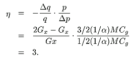
_x if the point elasticity of demand evaluation at
G* has an absolute value greater than 3. For, if
G
_d and 2
G
_x were coincident, that elasticity,
h, would be given by

However, even where
G
_d lies to the left of 2
G
_x, as in Figure 4.7, the perfectly discriminating solution may still be preferred. The gain from the move to the perfectly discriminating solution is the shaded area to the left of
D
_g between 3/2(1/
a)
MC
_g and (1/
a)
MC
_g, and has to be compared with the area of the shaded triangle between
G
_d and 2
G
_x below (1/
a)
MC
_g, which is the loss from possibly excessive government spending. (It can, in fact, be shown that the perfectly discriminating solution will be preferred if the point elasticity of demand at
G* is greater than ¾.)

Care must be taken in the analysis throughout to avoid confusion between the taxpayer’s anticipated demand for
G, the public good, and his anticipated demand for tax-base commodities,
A, B, or
X in our discussion, and depicted in Figures 4.1, 4.2, 4.4, 4.5, 4.7, and 4.8. Only in Figures 4.3 and 4.7 and the associated discussion are demand schedules for the public good depicted. In the discussion immediately above, the perfectly discriminatory solution serves to eliminate all potential consumer’s surplus in the purchase-use of the tax-base commodity,
X. But, by lowering the effective cost-price for the public good,
G, through the elimination of all excess burden in taxing
X, consumer’s surplus involved in the “purchase-use” of
G is increased. And, given plausible values of relative elasticity coefficients, it is conceivable that the taxpayer-consumer may prefer the discriminatory tax solution to the nondiscriminatory one.

At this point, we note an important difference between the model of the monopoly firm in price theory and our model of Leviathan as tax gatherer. In the former, the effective value of the analogue of
a is zero—that is, the consumer is not conceived as being a beneficiary of any part of the profits that the monopolist secures, and hence no value is placed by the consumer on any addition to such profits. The consumer would never voluntarily give up the net surplus that a shift from simple to discriminating monopoly would involve. In the Leviathan model, by contrast, the taxpayer does place some positive value on increments to monopoly tax revenues, because some proportion,
a, of them is spent on things (public goods) that the taxpayer values; and the parameter
a must take a positive value if any taxing power is to be granted to government at all.

It is interesting to note, however, that beyond the requirement that
a be positive, its value plays no direct role in the foregoing analytics at all: everything hinges on the elasticity of the demand curve for public goods. In some ways, this is a slightly surprising result because it seems to imply that the value of the increment to revenue that the move from proportional to perfectly discriminatory taxation generates is independent of the proportion of that revenue expended on public goods. However, this apparent anomaly is explained by the fact that the parameter
a exercises a similar influence on both the value of the incremental units of
G and the units originally allowed for under the proportional tax structure alternative. To the extent that
a does exercise an influence on this calculation, it does so indirectly and in a slightly surprising direction. The smaller
a is,
ceteris paribus, the higher the price and hence the smaller the quantity of
G within the neighborhood of which the extension of public-goods supply occurs. It seems reasonable to presume that, as in the case of a linear demand curve, the elasticity of demand will be higher in this range. In this sense, the smaller the proportion of revenue spent on public goods, the greater the likelihood that the citizen will desire the extension of revenue that the shift from a proportional to a perfectly discriminatory rate structure makes possible.

The results of this section contrast strikingly with those which emerged under other forms of discrimination examined earlier. If there is discrimination among individuals or among commodities, but not over units (because, say, of a requirement that rate structures be proportional), excess burden is directly related to maximum revenue, and the comparison of alternative tax bases can be conducted in terms of maximum revenue comparisons alone. Once discrimination over units is allowed, however, excess burden issues do obtrude. An increase in maximum revenue yield when the initial revenue yield is “appropriate” may indeed be desirable if that revenue increase results from a change in rate structure, from proportionality to regression.

Analogously, a reduction in revenue when revenue is “excessive,” achieved by restrictions on the rate structure—requiring progression, perhaps, or outlawing regression—cannot be unambiguously designated as desirable.

A second aspect of these results merits emphasis. It is clear that, at the constitutional level, the individual would prefer a perfectly discriminatory tax regime to a proportional tax that generates the same revenue yield. Suppose, for example, in Figure 4.6, that there is some potential tax base,
Y, the demand curve for which is identical with
AR
_x. The proportional tax on
Y would achieve the same maximum revenue as the perfectly discriminatory tax on
X, but would do so at 50 percent higher cost in terms of surplus forgone.

As in the earlier case with our discussion of possible discrimination in rates among taxpayers but not over quantities, the practical relevance of the whole analysis should not be overly emphasized. For the same reasons there mentioned, and others, effective rate discrimination over quantities may prove impossible to enforce for ordinary commodities. Even if interpersonal trades to implement indirect purchases could be prevented, the prospect for storage could allow single purchasers to take full advantage of the quantity discounts that the idealized differential rate structure would offer to the taxpayer. The possibility of any enforceable and effective differentiation over quantities purchased would be limited to nonstorable commodities.

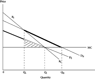Figure 4.8

Uniformity among persons, discrimination over units of commodity.  To complete the discussion of this section, it is interesting to examine briefly the case in which there is uniformity of treatment as among individuals, but where regression in the rate structure is allowed. We might conceptualize this setting as one in which constitutional-legal rules dictate uniformity of treatment among persons, but where differentiation in rates of tax over units is allowed as long as all persons face the same “offer schedule.” What rate structure will generate maximum revenue under these conditions? To answer this question, consider Figure 4.8. The simple two-person setting is again used, with
D_I and
D_II being the demand curves of individuals I and II for commodity
X. Under the constraint that I and II must be treated identically (i.e., they must face the same rate structure), it is clearly possible for II to be treated “as if” his demand curve for
X is
D_I; it is equally clearly impossible for I to be treated as if his demand curve were
D_II, because
D_I lies inside
D_II throughout. The revenue to be obtained from a single perfectly discriminating rate structure based on
D_I is given by the area between the new curve
R_I and
MC;
R_I is constructed so that the vertical distance between
R_I and
MC at any output is twice the vertical distance between
D_I and
MC. The revenue to be obtained from a single perfectly discriminating rate structure based on
D_II is the area under
D_II above
MC. A rate structure geared to discriminate ideally along
D_II would, of course, have the effect of eliminating the first person (I) from the market completely. The revenue-maximizing Leviathan will, if limited to these two options, choose between these solutions on the basis of revenue yield.

However, government will not in general find it revenue maximizing to focus on one or the other demand curve entirely. What is relevant here is the upper “envelope” combining the
R_I and
D_II curves. Up to the quantity level
Q
_s, where
R_I and
D_II intersect, more revenue is obtained by pricing according to
D_I; beyond that point, revenue will increase if there is a switch to
D_II and government levies a tax rate that just induces II to purchase additional units of
X. For instance, consider the output unit immediately beyond
Q
_s. If government levied taxes according to
D_I, the marginal revenue would be
R_I, which is less than
D_II in this range. The rate structure is, then, that depicted by the heavy line in Figure 4.8. It follows
D_I to
Q
_s and
D_II thereafter. It is therefore “regressive” over the ranges zero to
Q
_s and
Q
_s to
Q_II, but there will be a sudden discontinuous jump in rates at
Q
_s.

It is of some interest to compare the welfare loss in terms of excess burden per dollar of revenue in this solution with that in the various other discriminatory solutions previously examined, over commodities or individuals. We can show easily that the excess burden is indeed smaller here. For it will be recalled that, under maximum revenue assumptions, in all the cases where discrimination over quantities to individuals is not allowed, excess burden is exactly one-half of maximum revenue. In the case under examination here, however, such discrimination is all that is allowed. For individual I the excess burden is the shaded area under
D_I between
Q
_s and
Q_I (Figure 4.8). Because
R_I lies above
D_I but below
D_II over this range, this excess burden is less than one-half of the revenue raised from II over that range (from
Q
_s to
Q_I); since more revenue than this is raised
in toto, excess burden must
a fortiori be less than one-half of revenue over the entire range zero to
Q_II. And there is no excess burden on individual II since he purchases the same quantity under the tax structure postulated and under the no-tax market solution. The general conclusion, therefore, is that, under maximum revenue assumptions, the possibility of discrimination over units of the taxed good by means of the appropriately “regressive”
*59 rate structure provides a means of achieving revenue “more efficiently” (i.e., at smaller welfare loss per dollar of revenue raised) than does the completely nondiscriminatory alternative. Discrimination among goods and individuals in the absence of discrimination over units of output does not exhibit this property. Furthermore, this “efficiency” advantage of discrimination within the rate structure confronting each person does not depend on the presence or absence of other forms of discrimination.

It seems, on this basis, that the same conclusions hold here as with the perfectly discriminating regressive rate structure examined above. A uniform proportional tax may be dominated in the constitutional calculus by a tax that gains the same maximum revenue by means of an appropriately chosen rate structure that declines over units but is uniform among persons, applied to a smaller base. The desired level of revenue will be larger in the latter case, because total costs of public goods are lower due to the lower excess burden. It is possible that a tax which raises “too much” revenue under a uniform proportional rate will raise “too little” under a uniform “regressive rate” structure, even though revenue in the second case will be larger than in the former.

4.7. Summary

To an extent, this chapter has involved tying up many “loose ends” in comparative tax analysis and in particular application to commodity taxation. The comparative framework, which has allowed us to examine the explicit Leviathan model of our own construction in juxtaposition with the implicit benevolent despot of the conventional tax theory, necessarily introduces considerable complexity into the analysis, perhaps more than seems warranted for any straightforward presentation of the basic points. Comparisons with tax orthodoxy aside, the analysis of commodity taxation under our Leviathan assumptions becomes an extension of essentially the same logical construction developed with reference to income taxation in Chapter 3. The normative argument for tax-base restriction or limitation and against tax-base comprehensiveness is identical in the two separate fiscal institutions. The implicit orthodox argument for idealized rate differentiation among income sources is less familiar than the similar argument for idealized rate differentiation among differing commodity bases, largely because equity issues are allowed to enter more directly into the income-tax analysis. Nonetheless, the dramatic change in normative results produced by a shift to a government model of Leviathan applies equally to the two cases. The requirement for uniform treatment among persons in the income tax as well as the requirement for uniform rates of commodity taxation become instruments for limiting governmental fiscal appetites, instruments that may become relatively “efficient” when examined from the individual taxpayer’s genuine constitutional perspective.

The comparative analysis of the chapter has its own by-product advantages. It enables us to show how the equi-revenue setting of orthodox tax theory can be transformed into a useful analytical device even in a Leviathan model of government. When two tax instruments, exploited to produce maximum revenues, provide government with equal revenue yields, the traditional excess burden norms come into their own. In this context, however, the analysis suggests that there is a direct relationship between maximum revenue and excess burden. Under standard assumptions of linearity, equal maximum revenue taxation will generate equal excess burdens. Allowing departures from this linearity assumption would, of course, modify this precise relationship. But such complexity would do nothing to undermine the basic thrust of our analysis here.

Like Chapter 3, the discussion of Chapter 4 may be interpreted as a series of exercises in applied price theory. As noted previously, the assignment of a power to levy tax on a commodity base is fully analogous to the award of a monopoly franchise in the sale of a good. Price theory proceeds from the analysis of simple monopoly to that monopoly which finds it possible and profitable to engage in varying degrees of price discrimination as among markets, persons, and over quantities. As this chapter’s discussion has indicated, essentially the same logical catalogue can be applied to the taxing power, with essentially the same results if properly interpreted.

Appendix

The purpose of this appendix is to extend the analysis of Section 4.4 to a simplified general equilibrium approach somewhat more in keeping with the modern optimal-tax literature. Consider, for example, one of the simpler and more familiar discussions, that provided by Harberger.
*60 The tax rule derived by Harberger is designed for minimizing the welfare loss of a system of excises, given a revenue constraint, in a three-good setting in which one of the goods (leisure presumably) is tax-free. Let
X₁,
X₂, and
X₃ be the three goods, following Harberger’s formulation, and suppose
X₃ to be tax-free leisure. Then the change in
X₁ and
X₂ in response to taxes
t₁ and
t₂, respectively, is given by

	(1)
	(2)

where the units of
X₁ and
X₂ are chosen so that the initial prices are unity. Using the expression for the welfare loss as

(3)

we obtain

(4)

where

is the Hicksian substitution effect.

In the Harberger case,
W is minimized with respect to
t₁ and
t₂, given a revenue constraint. Harberger does not allow for the effect of changes in the tax base on revenue, but this can be done without changing the nature of his solution. For we seek to minimize

(5)

where

(6)

This becomes

(7)

The minimization exercise yields a set of equations

	(8)
	(9)

which solve to yield the optimal-tax structure,

(10)

(Harberger manipulates this to get

(11)

where
h_ij is the elasticity of demand for the
ith good with respect to the
jth price.)

For our purposes, however, we note that
R is given by

or

(12)

So to maximize
R with respect to
t₁ and
t₂ yields two equations:

	(13)
	(14)

which have the solution

(15)

which is precisely identical to Harberger’s tax rule, (10) above.

We note further that the left-hand side of (13) is
DX₁* from (1), and the left-hand side of (14) is
DX₂* from (2). So we have

	(16)
	(17)

and multiplying (16) by
t₁*, (17) by
t₂*, and adding, we have

or

(18)

from (3) and (6).

We can on this basis conclude that optimal-tax rules and maximum revenue rules are indeed identical, even in this simple general equilibrium setting; and further, that under maximum revenue assumptions, total revenue remains exactly twice the welfare loss, just as in the partial equilibrium case, even where discrimination between goods is permitted and general equilibrium effects allowed for.

52.

Conventional measures of excess burden focus on the second term of a Taylor series expansion of utility functions. That is, if we can represent individual utility functions as
U =
f (
X₁,
X₂, … ,
X
_n),then
which on manipulation can be shown to yield
[See Harberger, “Taxation, Resource Allocation and Welfare”; and Harold Hotelling, “The General Welfare in Relation to Problems of Taxation and of Railway and Utility Rates,”
Econometrica, 6 (July 1938), 242-69.] By taking higher terms of the Taylor series expansion, one can of course get more accurate measures of utility change. This is tantamount to allowing for differential curvature of demand (or marginal valuation) curves. So doing would permit a ranking of equi-maximum-revenue taxes according to total welfare loss but would involve measuring “excess burden” with a degree of refinement not used elsewhere in the literature and would in any case involve dealing with a high order of “smalls.”