Of all the things that puzzle me about macroeconomics, the relationship between changes in monetary policy and changes in long-term interest rates is perhaps the most confusing. I get why monetary injections tends to reduce short-term rates—-prices are sticky and short-term rates temporarily fall to equilibrate monetary supply and money demand, until prices have time to adjust. But prices are not sticky for 30 years.
I also notice that persistent periods of easy money (such as the 1960s and 1970s) leads to higher interest rates, and periods of tight money like 1929-33 lead to lower interest rates.
What confuses me is that (unexpected) easy money announcements will sometimes raise long-term rates (as in January 2001 and September 2007) and at other times easy money shocks will cause long-term rates to fall, as in the market response to the recent moves by the Bank of Japan. And here is what’s even stranger; in both cases stock prices soared. Stocks soared as long-term bond yields rose in response to easy money announcements in January 2001 and September 2007, and stock prices soared in response to easier money in Japan that lowered long-term interest rates. This suggests that stocks are responding to the easy money itself, not the impact the easy money has on long-term bond yields.
I find my inability to understand why easy money sometimes raises rates and sometimes lowers rates to be very frustrating. But now I have an idea that might make the problem at least slightly less mystifying. When mathematicians are struggling to prove a difficult theorem, they will sometimes look for connections with other theorems that are better understood. Let’s translate the “response of long-term bond yields to money shocks puzzle”, into another area of economics, which is much better understood.
Back in 1975, Rudi Dornbusch showed that an easy money policy would cause exchange rate “overshooting”. The argument went as follows: Easy money would reduce domestic interest rates. Because of the interest parity theorem, lower interest rates imply a higher rate of appreciation of the domestic currency over time. (For simplicity, assume the interest rates in both countries were originally equal.) But the quantity theory of money implies that the easy money will raise the price level, at least in the long run. And purchasing power parity implies that the higher future price level will lead the exchange rate to depreciate, again in the long run. So how can the exchange rate be expected to both appreciate and depreciate? Dornbusch showed that it would do so by overshooting its long run equilibrium. Thus an expansionary money announcement might cause the exchange rate to instantly fall by 5%, and then gradually appreciate by 3%, still ending up 2% lower than the original exchange rate.
I’d like to translate the money shock/long bond yield puzzle into the language of the interest parity theorem. To do so, I’d like you to consider a central bank that does not use the interest rate as its policy instrument (as the Fed does) but rather uses the exchange rate as its policy instrument. More specifically, I’d like you to consider two policy options for the Singapore central bank, which does use exchange rates as a policy instrument:
Option A: A policy of suddenly depreciating the currency by 5%, but then promising to gradually appreciate it afterwards at a rate 0.1% higher than was previously expected.
Option B: A policy of suddenly depreciating the currency by 5%, and then promising to gradually depreciate it afterwards at a rate 0.1% higher than was previously expected.
These are both expansionary monetary policies. Both policies are clearly feasible for the central bank of Singapore. And yet option A lowers long-term bond yields by 0.1%, while option B raises long-term bond yields by 0.1%.
If you are very smart, like a Paul Krugman or a Nick Rowe, you are probably bored stiff by this exercise. “Tell me something new.” But for me this new framing helps to clarify some issues. Now I can think about what sort of policy regimes might lead to each of the two outcomes. Under a Bretton Woods type regime, with a gold price peg, one might view any easy money policy as likely to be temporary. Then you get option A occurring. And since that type of regime describes most of our history, it’s no surprise that the “liquidity effect” (i.e. easy money leads to low interest rates) is the normal way that most people look at monetary policy.
On the other hand when there’s a lot of uncertainty about the future path of policy, option B might occur more often. Easy money leads to fears of inflation, and higher long-term bond yields.
This exercise also clarifies that the puzzle I opened the post with is essentially a “levels vs. growth rates” puzzle. Monetary policy can be thought of as working in two dimensions: changes in the price level, and changes in the rate of inflation. We don’t see this clearly because most prices are sticky, so even level shifts look a lot like growth rate shifts. But one price is not at all sticky—exchange rates! They are sort of the canary in the coal mine; showing you what the impact of a monetary policy shock would be in the long run. Think of the exchange rate as a sort of “shadow price level”, showing what changes in the price level (in response to monetary shocks) would look like if prices were not sticky.
Because monetary policy operates in terms of both growth rate and level shocks, it’s really complicated. But what makes it far, far more complicated is that the interest rate (which can go either way) is also used as a policy instrument. So now investors need to figure out how a given change in the target interest rate will:
a. Impact the expected future path of short-term interest rates, relative to a natural interest rate that is itself influenced by the path of monetary policy.
b. How the current change in interest rates, and the change in the future path of short-term rates relative to the natural rate, will influence the current and expected future path of exchange rates.
c. How the change in the expected future path of exchange rates will impact current long-term bond yields.
Notice that the last step is a sort of afterthought. Easier money will have its effects (lower exchange rate, higher inflation, more jobs, more NGDP, higher stock and commodity prices, etc.) regardless of whether long-term rates rise or fall in response to easier money. Long rates are just an epiphenomenon.
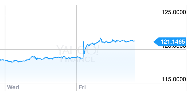
This post doesn’t really solve anything, but for me it makes the mystery a bit less confusing. For instance, look at the response of the yen to the recent BOJ announcement:
Notice the zigzag immediately after the announcement. I recall a similar pattern for US stock indices right after the September meeting, where the Fed failed to boost rates. In my view this uncertainty is caused by the incredible complexity of monetary policy.
Remember that the market is like a giant brain, far smarter than any individual. So the fact that even it has trouble figuring out this levels/growth rate problem shows just how confusing monetary policy actually is. Still, the market gives us the best estimate we have for the effects of monetary policy.
Some commenters argued that markets can be irrational and that the tendency of currencies to depreciate after negative IOR, or QE, might be an irrational response. They say it “doesn’t prove anything”. What they forget is that the exchange rate is itself an important macro variable. If easier money causes exchange rate depreciation, then easier money is effective at boosting prices and NGDP, even if the market is completely stupid in driving exchange rates lower. Perhaps markets never studied Post Keynesian endogenous money theory. But even if the market is in some sense “wrong”, its beliefs become self-fulfilling.
I believe that in the 21st century, macro will be increasing seen as a field focused on stabilizing various market price indicators, and that people like Roger Farmer will be increasingly influential, even though his approach (focusing on stock prices) is somewhat different from my obsession with NGDP futures prices.
READER COMMENTS
Nick Rowe
Feb 1 2016 at 5:51pm
I’m only smart enough to think: “I wish I’d thought of that thought-experiment”.
John Hall
Feb 1 2016 at 7:38pm
Good post.
Philo
Feb 2 2016 at 9:55am
Another brilliant post. Can you keep this up? (Granted, you have to take praise from a non-economist with a grain of salt.)
maynardGkeynes
Feb 2 2016 at 8:27pm
Could it be that the robots that you refer to as “the stock market” are programmed to use short term rates rather than long term rates as the discount rate plugged into the Gordon equation?
AbsoluteZero
Feb 2 2016 at 10:00pm
This paragraph, really just the last sentence, needs to be repeated, everywhere.
One of the things one learns upon entering finance, especially from a highly precise tehnical field, is that the whole system is fundamentally self-fulfilling.
Brian Donohue
Feb 3 2016 at 9:36am
Superb post, Scott. Worth meditating on. Deep waters.
Scott Sumner
Feb 3 2016 at 10:02am
Thanks everyone, and Nick’s being too modest; he has far more clever thought experiments than I do.
MaynardGKeynes, I think of individual robots as like individual brain cells. Each individual cell in a brain is stupid, but the collection of cells is wise (insert political joke here.)
o. nate
Feb 3 2016 at 10:30am
Very interesting and clearly written. I’m not as confident as you are that the markets are able to digest information about macro policy direction so quickly and efficiently. In the case of Japan, it now looks like markets have retraced a lot of their post-announcement moves in the yen and Nikkei as Japanese bank stocks have tanked.
dlr
Feb 3 2016 at 9:18pm
I love this post. I’m confused about how overshooting solves the equilibrium problem between interest rate parity and the Fisher equation. Your country A has seen an immediate forex depreciation of 5%, but now expects .1% higher appreciation than before. So let’s say it overshot what was really a 2% long-term expansionary policy and after 30 years it will go back the preexisting appreciation/depreciation rate but at a permanently 2% lower forex rate. This presumably also means that the price level is 2% higher than it otherwise would have been assuming RER are unchanged. But the price level hasn’t moved at all on the announcement because it is sticky.
Doesn’t this mean that bond yields (30 yr, 10 yr, anything outside of the sticky price period) should still rise on the announcement (yes, contra interest rate parity) given sticky prices and the Fisher equation? Why would someone accept a lower rate on a long term bond given a higher expected future price level change over 10 or 30 years?
Brian Donohue
Feb 6 2016 at 10:22am
Scott,
Any reaction To the paper Fama just wrote?
http://raps.oxfordjournals.org/content/3/2/180.full.pdf+html
I thought it was good. Not Earth shattering, but thoughtful and careful.
Comments are closed.