Accounting for Capital and Income

Our three examples highlight the importance of understanding both the theory and the practice of capital and income measurement. Analysts have often used statistics to make statements about U.S. savings behavior and inequality, without understanding some important causes of the observed outcomes. This article will help the reader to avoid such pitfalls and interpret the empirical evidence more knowledgeably. In particular, changes to the tax code in the 1980s drastically altered the reporting of various types of income, even though the underlying income levels probably did not change nearly as much. This fact is highly relevant in today’s policy disputes, because a pioneering indicator of growing wealth inequality is based on income tax data. It is entirely possible that the apparent surge in wealth inequality is largely spurious, reflecting large changes in the tax code but not large changes in the underlying economic reality.

Two Perspectives on Capital and Income

There are two ways to think about the connection between capital and income. On the one hand, if we have an asset that we expect to yield a certain flow of payments in periodic bursts over time, we can compute its capitalized market value by summing up the present discounted value of the entire stream of expected future payouts. In this approach, the flow of income is the more fundamental or “primitive” concept, upon which the derivative idea of capital is built.

As an example of this first approach, suppose that an investor considers purchasing a parcel of downtown real estate that includes an apartment building. The investor estimates that, after accounting for routine maintenance and other administrative expenses, the rent he will collect from tenants will yield him a net income of $100,000 per year, a situation he expects to last indefinitely.

Under these assumptions, at a 10-percent discount rate, the investor would be willing to pay up to $1 million for the property, while at a 5-percent discount rate, he would be willing to pay up to $2 million. This type of analysis shows the sense in which the underlying “fundamentals” are the origin of the market value of the wealth; it’s not as if the investor’s capital investment in the property would automatically generate a return of 5 or 10 percent. On the contrary, the original market price of the property adjusts so as to make the expected return (all things considered, including uncertainty) on the apartment building comparable to the return on other such investments.

Although the capitalization method that we have just discussed is intuitive, Friedrich Hayek, in his monumental Pure Theory of Capital, took a different view. He started with capital as the fundamental concept. He defined income as the flow of consumption generated by a collection of capital goods that one could enjoy in a certain period, without impairing the future productive power of the capital.1 This approach is useful for dealing with change.

For example, suppose that the above investor, using the market discount rate of 5 percent, plunks down $2 million to buy the real estate containing the apartment building. As predicted, in the first year, the asset generates $100,000 in net income. However, during the second year, the investor learns that several of the trees on the property have become infested with an insect and that, without corrective action, some of the trees will eventually topple into the building. Because the investor wants to protect the physical integrity of the building and thereby ensure its financial ability to continue to provide a flow of rental payments from tenants, he pays $15,000 to have the infected trees removed and replaced. Thus, his net income for the second year is only $85,000. Note that, in the second year, the owner actually received the same gross payments from his tenants as in the first year; he could have withdrawn the full $100,000 from the operation. Yet such shortsighted behavior would have reduced future flows of income from the capital asset. Had the owner spent the full $100,000, he would have been “consuming capital.”

This discussion helps us appreciate Ludwig von Mises’ remarks on “calculation,” which was his term for the mental procedure by which money prices guide individuals in a market economy:

Monetary calculation reaches its full perfection in capital accounting. It establishes the money prices of the available means and confronts this total with the changes brought about by action and by the operation of other factors. This confrontation shows what changes occurred in the state of the acting men’s affairs, and the magnitude of those changes; it makes success and failure, profit and loss ascertainable. The system of free enterprise has been dubbed capitalism in order to deprecate and to smear it. However, this term can be considered very pertinent. It refers to the most characteristic feature of the system, its main eminence, viz. the role the notion of capital plays in its conduct.2

The capital Gain (or loss): Where the Two Perspectives Unite

In the previous section, we saw that there are two ways to view the relationship between capital and income: In a static framework, where we can perfectly anticipate the magnitude and timing of future income yielded by an asset, its capital value will simply be the present discounted value of those future cash flows. In a dynamic framework, we can calculate the income (or loss) associated with an operation by the change in the capital value of its components.

These two perspectives come together in the concept of a capital gain (loss), which is a type of income. Consider, again, our real estate investor, who uses a 10-percent market discount rate and invests $1 million in an apartment building. A few years after the purchase, a new opera house opens down the street, making the neighborhood much more desirable. Consequently, the investor raises his tenants’ rent and ends up netting $200,000 annually, after maintenance expenses. If this is now the “new normal,” at the same 10-percent market discount rate, the capitalized value of the property jumps to $2 million. (From that point forward, the $200,000 annual net rental income represents a 10-percent return on the invested $2 million of capital.) Thus, the investor enjoys a $1 million capital gain the moment the new reality sinks in.

For a different example, consider the original scenario again—i.e., the investor earns $100,000 in annual net income from his tenants. Now suppose that the market rate of interest suddenly falls from 10 percent to 5 percent. Even though the expected flow of annual net rental income remains the same, its present discounted value immediately jumps from $1 million to $2 million. (From that point forward, the $100,000 annual net rental income represents a 5-percent return on the invested $2 million of capital.) The $1 million difference registers as a capital gain, accruing (in a theoretical sense) the moment interest rates fall.

It’s important to stress that capital gains are actually income, in an economically meaningful sense. In either of the above scenarios, the investor could have sold his property for $2 million cash, even though he had initially put only $1 million into it. There was, thus, a real sense in which the “amount of capital invested in the operation” jumped from $1 million to $2 million as soon as people in the market processed the new information.

Economic Theory versus Empirical Measures

Although in theory, the connection between capital and income can be spelled out quite elegantly, in practice, discussions of these concepts are severely limited by the availability of data. In this section, three examples highlight the pitfalls in relying on popular statistics of capital or income to draw conclusions about the economy.

For the first example, consider the “personal saving rate,” which began a long slide in the early 1980s and reached historical lows by the mid-2000s, as shown in Figure 1:

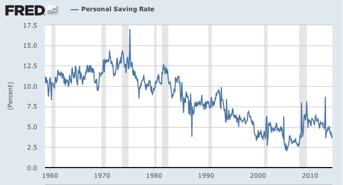
Analysts could (and did) come up with various explanations for the trend shown in Figure 1, often blaming the policies of the presidents in office as the personal saving rate fell. Yet, before discussing Figure 1, it is crucial to understand that the definition of personal income used by the Bureau of Economic Analysis (BEA) excludes capital gains in both real estate and stock equity.3

The BEA’s decision is defensible since it ties its definition of “personal income” to the national income accounts; if the stock market rises by $1 trillion, that does not count as part of GDP because that $1 trillion does not reflect an increase in production. Even so, the drop in the BEA’s “personal saving rate” in Figure 1 can be very misleading, as it occurred during a period when millions of Americans, especially baby boomers, started using tax-qualified plans, such as Individual Retirement Accounts (IRAs) and 401(k) accounts, to buy stocks. Furthermore, the low personal saving rate in the 2000s was undoubtedly influenced by the booming housing market: If someone’s home value unexpectedly rose $20,000 in a year, that would make her less eager to save as much out of her wage or salary income. (Of course, the housing crash would later make many such homeowners regret their earlier decisions.)

The second example focuses on the distinction between capital gains and realized capital gains. Economic theory says that a capital gain accrues the moment new information hits. In practice, however, tax laws and, hence, the tax returns on which empirical studies are based, typically require capital gains to be recognized as income only when they are actually realized. For example, if an investor buys a stock at $100 in 2014, holds it as it rises to $120 in 2015, and finally sells it at $120 in 2016, then, when she files her 2016 taxes, she reports a $20 capital gain. She doesn’t report the $20 capital gain in 2015, even though that’s when it accrued.

Because of this feature of the tax treatment, changes in the capital gains tax rate can have huge effects on reported capital gains. For example, in 1986, there was a significant overhaul to the tax code that resulted in (among other things) a less favorable treatment of capital gains. As one analyst explains it:

Throughout this process, the designers of the 1986 Act … recognized that the significant reduction in the capital gains preference could raise questions of fair transition. Accordingly, they wrote the law with a prospective effective date (January 1, 1987), so that taxpayers who had contemplated selling assets using the prior law preference would have a window to do so. This, of course, created a “fire-sale” opportunity for realization of gains at what was in effect a temporarily low rate.4

To see the enormous impact of the 1986 change, as well as the effects of other capital gains tax rate changes, consider Figure 2:

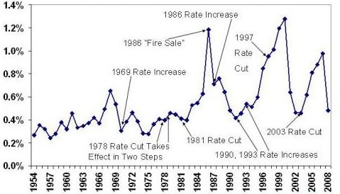
As Figure 2 should make clear, any discussion of capital income that relies on tax data must take into account the effect of rate changes on the decision to sell assets and realize accruing capital gains. Someone who did not understand the concept of a “realized capital gain” might be very disappointed in how little revenue came in after a hike in the capital gains tax rate. It is much easier for the owners of financial assets to time the realization of their income gains compared to, say, salaried workers adjusting the timing of their earnings in response to changes in the tax code.

The final example draws on several of the issues discussed thus far. In the controversy over the work of Thomas Piketty and his bestselling Capital in the Twenty-First Century, one of the key pieces of evidence is an unpublished (as of this writing) analysis by Emmanuel Saez and Gabriel Zucman showing that the percentage of total wealth held by the richest 0.1% of Americans has surged since the mid-1980s to levels not seen since the 1920s.5 Far from apologizing for his decisions regarding data sources and how to blend them, Piketty now claims that the Saez-Zucman findings show that, in his book, he (Piketty) had been too modest.6

Ironically, the new blockbuster Saez-Zucman findings contradict the flat trend of wealth inequality that Saez himself (with a different co-author, Wojciech Kopczuk) published in 2004.7 In their PowerPoint slides, Saez-Zucman highlight this inconsistency, shown here in Figure 3:

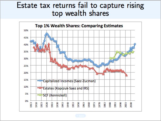
Figure 3 shows that the two approaches of Saez and his respective co-authors matched pretty closely for most of the 100-year history, except for a divergence that began in the late 1980s. The Kopczuk-Saez (2004) series—shown in red—indicates a fairly constant concentration of wealth in the hands of the top 1% for many years, starting in the late 1980s, and the most recent data point is the lowest concentration of wealth in the whole series. In stark contrast, Saez’s 2014 method (with co-author Zucman), shown in blue, shows the top 1%’s share of total wealth skyrocketing from the 1980s.8

What could explain this divergence? As the PowerPoint slide title indicates, Saez and Zucman believe it is simply that the estate tax data (the 2004 method) fail to catch the true rise in inequality; they take it for granted that their new measure is the one that accurately reflects the economic reality.

But there is another possibility. Although they have not released a paper showing their exact method, Saez and Zucman explain in their PowerPoint slides that their new approach takes various forms of income from tax-return data, then combines them with the rates of return by asset class from the flow of funds and NIPA data, to produce the total capitalized value of assets held by various portions of the population. For example, rather than directly measuring the size of an individual’s stock portfolio in a given year, the Saez-Zucman approach would look at how much dividend income the individual reported to the IRS that year, then use an estimate of the dividend rate of return in order to “back out” the size of the stock portfolio necessary to generate such a dividend income. The crucial point is that the new Saez-Zucman measure of wealth is actually based on income data collected by the IRS.

As I explained in the first section of this essay, there is a relationship between income and wealth, and so the new Saez-Zucman measure of wealth inequality makes sense on methodological grounds. However, there is a huge potential pitfall in their approach: Significant changes to the U.S. tax code in the 1980s changed the classification and reporting of income. That means the new Saez-Zucman method of estimating wealth may be very misleading when we look at its output pre- and post-1980s, because the IRS income data on which it is based are themselves incommensurable. Specifically, the sharp reduction in marginal personal income tax rates—with the top bracket dropping from 70 percent in 1980 to 28 percent by 1988—caused many high-income people to reorganize their businesses as pass-through entities (such as S Corporations) because it was now better to have this “business” income taxed as personal income rather than at the corporate rate. To the extent that the new Saez-Zucman technique measures wealth by capitalizing current income, therefore, their measure will overstate the increase in the top 1 percent’s wealth since the late 1980s. One reason, again, is that changes to the tax code in the 1980s made it advantageous for high-income individuals to shift income that previously had been reported as “business” income accruing to a corporation to now be classified as personal income accruing to an individual. This reclassification caused a surge in the apparent earnings of high-income individuals, even though their actual situation had not improved as much as these numbers suggested.

Furthermore, the rise of tax-deferred investment vehicles in the 1980s removed much of the middle class’s realized capital gains, dividends, and interest from the tax forms altogether because they were not taxable gains. Thus, middle-class income was artificially understated relative to income in the 1970s, when such gains were reported. When discussing studies of income (not wealth) inequality, Alan Reynolds points to these major changes in the tax code and writes, “[I]t is extremely deceptive to compare tax-based estimates of income distribution from 1970 to 1979 with any year after 1986.”9

In light of the major problems with tax-based measures of income inequality occurring in the 1980s, it is entirely possible that measures of the capitalization of this putative income—in other words, the new Saez-Zucman measures of wealth—are likewise tainted. The major changes that Reynolds outlines in his book go a long way to explain why tax-based measures of income could have skyrocketed after the 1980s, while tax-based measures of wealth remained flat. We should therefore be very skeptical of the income-based measures of wealth that skyrocket after the major tax changes in the 1980s, when the measures directly assessing estates show no such increase.

Conclusion

The relationship between capital and income is intuitive and elegant in a theoretical framework of perfect information. However, in a changing world with limited data sources, it is crucial for the analyst to understand the actual definitions and method underlying a particular series before drawing conclusions from it.